1. Expression

Let \(Y_{(i)}, i = 1,2, \ldots, n\) be the ordered sample from a region (can be division/district/thana), in our case, thana.

• Let \(M\) denote the number of observation less than the threshold \(L\) (given).
• Let \(F_n(x) = \frac{1}{n}\sum_{i = 1}^{n}I(Y_i \leq x), x \geq 0\), the empirical distribution be the estimator of true distribution \(F(x)\).

For arsenic (As) level \(Y_{(i)}\), the corresponding propensity socre, denoted by \(C_{ni}, i = 1,2, \ldots,n\) is given by

\[\begin{align} \tag{2.1} C_{ni} = \max(0, (1 - L/Y_i)^{\hat{\theta(Y_{(i)})}}) \end{align}\]

where

\[\begin{align} \tag{2.2} \hat{\theta(Y_{(i)})} = \frac{2}{n-M}\sum_{j = M+1}^{n}\frac{\min(Y_{(i)},Y_{(j)})}{Y_{(i)}+ Y_{(j)}}, i = 1,\ldots, n \end{align}\]

and finally the CSI is the mean of the propensity score averaged by all \(n\) observation.

\[\begin{align} \tag{2.3} \hat{C}_E = \frac{1}{n}\sum_{M \leq i \leq n}C_{ni} \end{align}\]

Note: For Equation (1), if \(Y_{(i)} \leq L\), then \(C_{ni} = 0\).

2. Implementation

propensity_score <-function(x, y_vector, L = 10){
  # x is argument, i.e. oberservation to be convert
  # y_vector is a vector of ALL observations in the sub_region
  
  n <- length(y_vector)
  y_truncate <- y_vector[y_vector > L]

  # case that ALL observation less than the threshold
  if(length(y_truncate) == 0)
    return(rep(0, n))
  
  # when num of y_trancate == 1, then 2/(n-M-1) = infinity
  if(length(y_truncate) == 1)
    return(max(0,1-L/x))
    
  # base of Eq. (1)
  C_ni <- max(0,1-L/x)
  
  # coeff * y_sum is Eq. (2)
  coeff <- 2/length(y_truncate)
  y_sum <- sum(pmin(x,y_truncate)/(x + y_truncate))
  
  # return value of Eq. (1)
  return(C_ni^(coeff*y_sum))
}

Once we have the CSI score for the thana, CSI is simply the mean of the scores of all observations.

csi <- function(y_vector){
  # find propensity score for each observation
  score <- sapply(y_vector, y_vector = y_vector, propensity_score)
  # mean of the score is csi
  return(mean(score))
}

3. Result

We present two type of plot,

• The first one we use the exact CSI values value computed from the estimator, it is presented in a continuous scale.

library(tibble)
library(ggplot2)
library(dplyr)
thana_obs <- split(dataset, dataset$thana_id)

thana_csi <- function(data_list, discrete = FALSE){
  n <- length(data_list)
  csi_vector <- rep(NA, n)
  ids <- names(data_list)
  for(i in 1: n){
  csi_vector[i] <- csi(thana_obs[[i]]$as)
  }
  cutoff <- seq(0, 1, length.out = 11)
  if (discrete == TRUE){
    csi_vector <- cut(csi_vector, breaks = cutoff, include.lowest = TRUE)
    csi_vector <- factor(csi_vector, levels = rev(levels(csi_vector)))
    }
  # can consider rounding to 3 decimals
  df <- tibble(id = ids, csi = csi_vector)
  return(df)
}

# csi in dataframe
csi_df <- thana_csi(thana_obs)
# plotting result
thana_df <- fortify(thana_map)
# merge result
plot_csi <- left_join(thana_df, csi_df, by = 'id')

dcsi_df <- thana_csi(thana_obs, discrete = TRUE)
plot_dcsi <- left_join(thana_df, dcsi_df, by = 'id')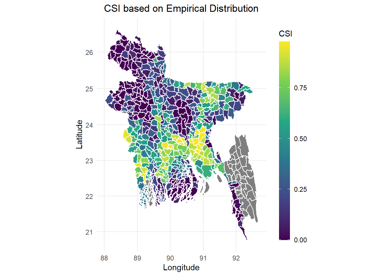

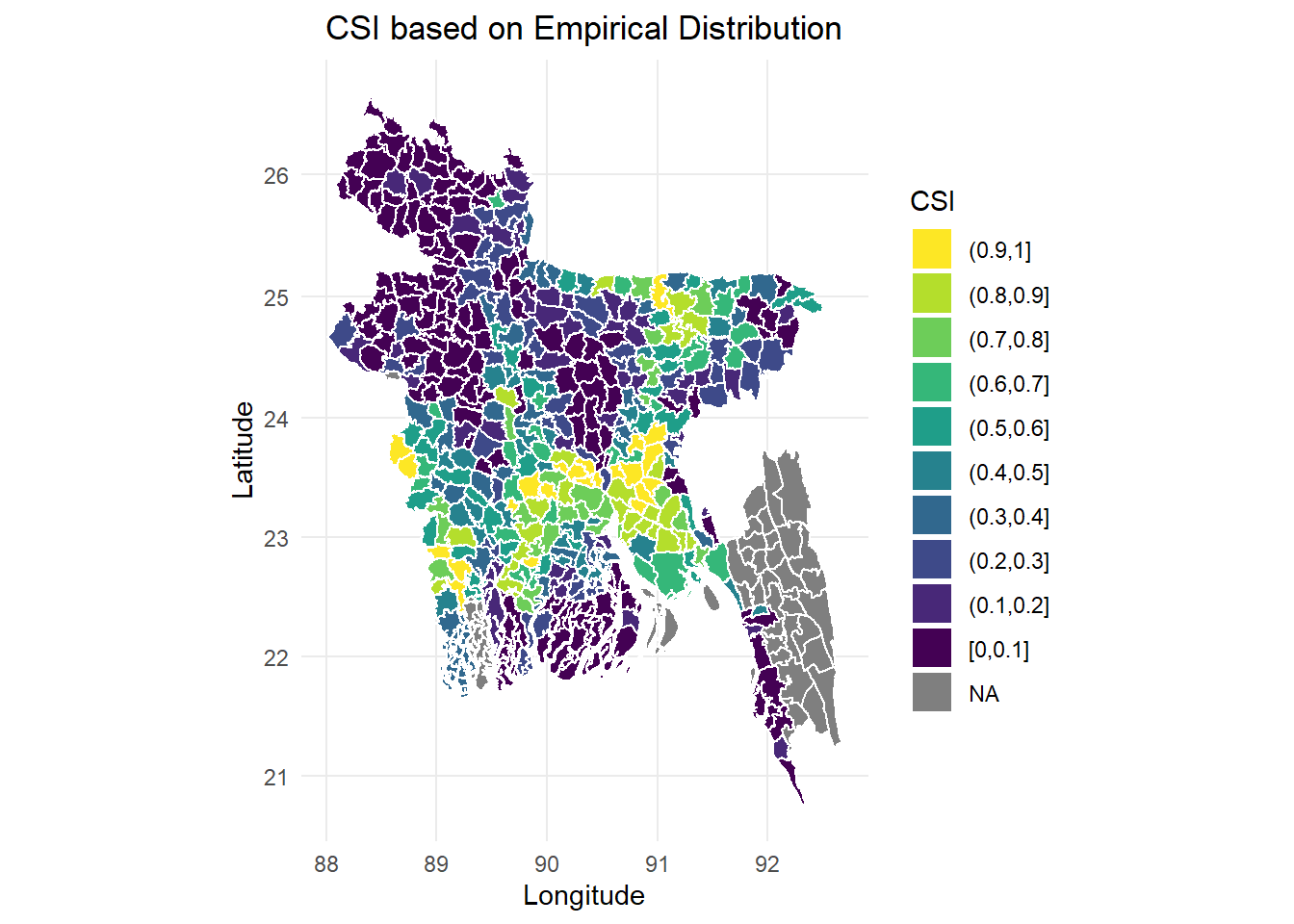
• The second one we use the exact 10 bins, from which we divide 0 - 1 into 10 categories, it is presented in a discrete scale.

References

1. Sen, P. K. (2016). Abundant Environmental Arsenic Contamination: Some Statistical Perspectives. Sankhya B, 78(2), 341-361.

2. Viridis Color Scales