1. Prelimineray

Example on CD4

In the following example, I will demonstrate fitting a LMM with missing data via rstan the data is obtaining from Dr. Patrick Breheny’s Bayesian Modeling in Biostatistics, according to the description, the data set contains repeated measurements on a sample of 251 children, each followed up for a period of one and a half years. In addition to CD4Pct, the data set also contains the following variables (I only include those I will use in the model):

• \(\texttt{CD4Pct}\): The concentration CD4 Cells.

• \(\texttt{ID}\): Each patient is assigned a unique ID. Note that there are several observations (rows) per patient.

• \(\texttt{Visit}\): Ideally, patients were supposed to have visits at 1, 4, 7, 10, 13, 16, and 19 months, with 1 month being the initial visit. As is always the case in hospital data like this, the “16-month” visit did not take place exactly 15 months after the “1-month” visit, but Visit provides a rough approximation to the elapsed time between visits. Note that not all patients have an observation for each visit.

According to the EDA, we find that the \(\texttt{CD4Pct}\) itself does NOT follow a normal distrubtion but the square root transformation will be solving this problem, hence we will use \(Y_{ij} = \sqrt{\texttt{CD4Pct}_{ij}}\) be response.

First we read and manipulate the data

library(dplyr)

cd4 <- read.delim("data/cd4.txt", header = TRUE)
n_obs <- nrow(cd4)

J <- max(cd4$ID)
x <- seq(from = 1, by = 3, length.out = 7)
df <- tibble(id = rep(1:J, each = 7), visit = rep(x, J))

cd4 <- cd4 %>% select(id = ID, visit = Visit, CD4Pct) %>% 
               right_join(df, by = c('id', 'visit')) %>% 
               mutate(y = sqrt(CD4Pct))

n <- nrow(cd4)                  

cd4_data <- list(N = n, N_obs = n_obs, y_obs = cd4$y[1:n_obs], visit = cd4$visit, id = cd4$id, J = J)

We consider a varying-intercept varying-slope model, we save the model in a stan file named cd4.stan, detail of the model is as follows,

data {
  int<lower=0> N;
  int<lower=0> N_obs;
  int<lower=0> J;
  vector[N_obs] y_obs;
  int visit[N];
  int<lower=1, upper=J> id[N];
}

transformed data{
  int N_miss = N - N_obs;
}

parameters {
  vector[N_miss] y_miss;
  
  vector[J] alpha;
  vector[J] beta;
  
  real<lower=0> sigma_y;
  real<lower=0> sigma_a;
  real<lower=0> sigma_b;
  
  real mu_a;
  real mu_b;
}

transformed parameters{
  vector[N] mu;
  vector[N_obs] mu_obs;
  vector[N_miss] mu_miss;
  
  for(i in 1:N)
    mu[i] = alpha[id[i]] + beta[id[i]] * visit[i];
  
  mu_obs = head(mu, N_obs);
  mu_miss = tail(mu, N_miss); 
}

model {
  mu_a ~ normal(0, 100);
  mu_b ~ normal(0, 100);
  
  sigma_y ~ uniform(0, 100);
  sigma_a ~ uniform(0, 100);
  sigma_b ~ uniform(0, 100);
  
  for(j in 1:J){
    alpha[j] ~ normal(mu_a, sigma_a);
    beta[j] ~ normal(mu_b, sigma_b);
  }
  
  y_obs ~ normal(mu_obs, sigma_y);
  y_miss ~ normal(mu_miss, sigma_y);
}

library(rstan)
# allow mutli core running at the same time to accerlate fitting process
options(mc.cores = 3)

fit <- stan(file='cd4.stan', data = cd4_data, chains = 3,
           iter = 2500, warmup = 2000, refresh = 1000, save_warmup = FALSE)

This will takes some time to compile the model and fitting MCMCs. This example takes about 45 second on my desktop. Once the fitting is done, we may extract the posterior samples and performing related analyses.

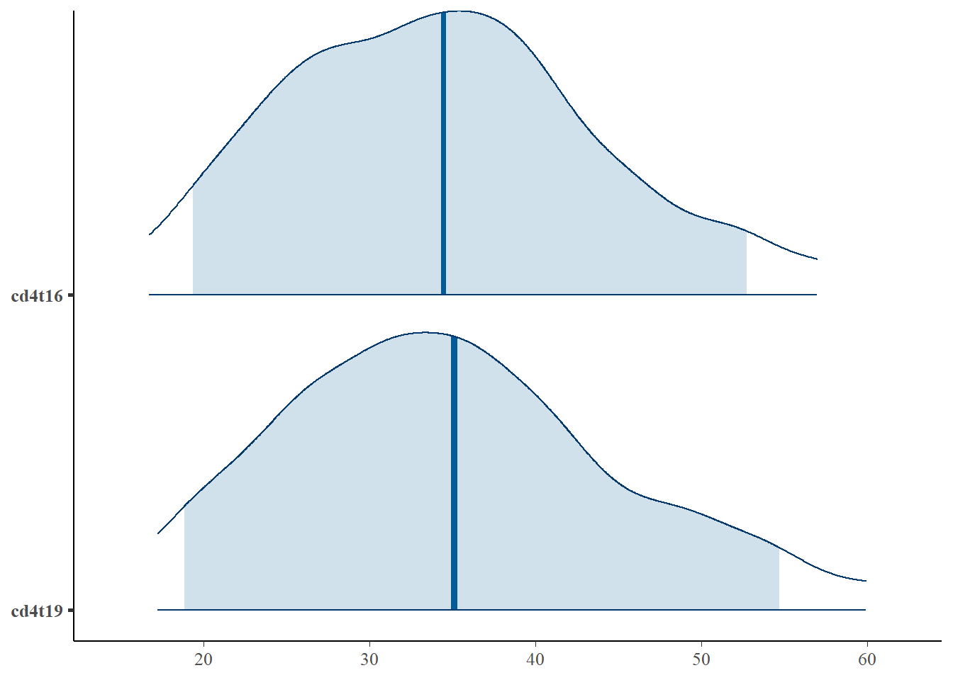
For example, we want to see the the prediction of missing response for ID = 18, also, we want to see the posterior distribution of the variance parameter \(\lbrace \sigma_y, \sigma_a, \sigma_b \rbrace\) by difference chains. The result can be plotted either by some built-in rstan function or a more flexible package called bayesplot.

idx <- which(cd4_data$id == 18)
idx[idx > cd4_data$N_obs] - cd4_data$N_obs

# position of y_miss for ID = 18
y18 <- extract(fit, pars = c('y_miss[38]', 'y_miss[39]'))
# permuted = FALSE, then will save data by chain
sigmas <- extract(fit, pars = c('sigma_y', 'sigma_a', 'sigma_b'), permuted = FALSE)

id18 <- tibble(t16 = post_param$`y_miss[38]`, t19 = post_param$`y_miss[39]`)
id18 <- id18 %>% mutate(cd4t16 = t16^2, cd4t19 = t19^2)

library(bayesplot)

mcmc_areas(id18, 
  pars = c('cd4t16', 'cd4t19'),
  prob = 0.9, # 90% intervals
  prob_outer = 0.95, # 99%
  point_est = "mean"
)

mcmc_dens_overlay(sigmas, pars = c('sigma_y', 'sigma_a', 'sigma_b'))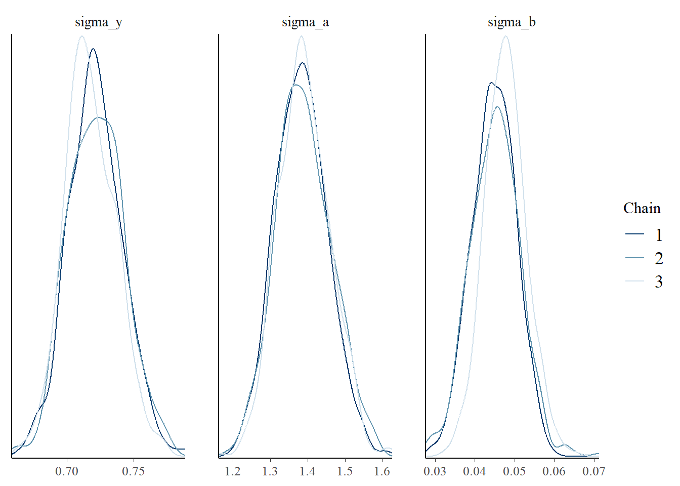

References:

1. Hoffman, M. D., & Gelman, A. (2014). The No-U-Turn sampler: adaptively setting path lengths in Hamiltonian Monte Carlo. J. Mach. Learn. Res., 15(1), 1593-1623.

2. Stan User Guide

3. bayesplot documentation